A General Recipe for Likelihood-free Bayesian Optimization

Abstract

The acquisition function, a critical component in Bayesian optimization (BO), can often be written as the expectation of a utility function under a surrogate model. However, to ensure that acquisition functions are tractable to optimize, restrictions must be placed on the surrogate model and utility function. To extend BO to a broader class of models and utilities, we propose likelihood-free BO (LFBO), an approach based on likelihood-free inference.

LFBO directly models the acquisition function without having to separately perform inference with a probabilistic surrogate model. We show that computing the acquisition function in LFBO can be reduced to optimizing a weighted classification problem, where the weights correspond to the utility being chosen. LFBO outperforms various state-of-the-art black-box optimization methods on several real-world optimization problems. LFBO can also effectively leverage composite structures of the objective function, which further improves its regret by several orders of magnitude.

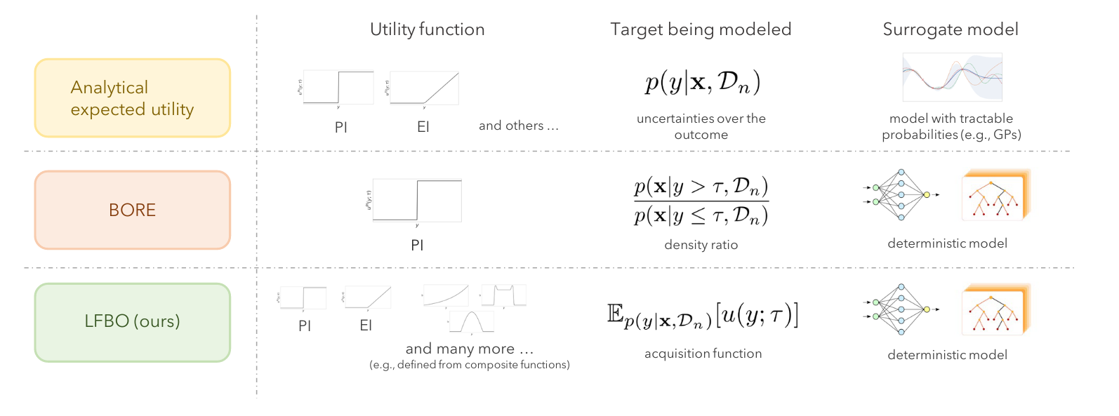
Acquisition functions as expected utility

Suppose we have an expensive and possibly-noisy black-box function $f$, i.e., we can query at a location $x$ and get $y = f(x)$ but we do not have additional information about $f$.

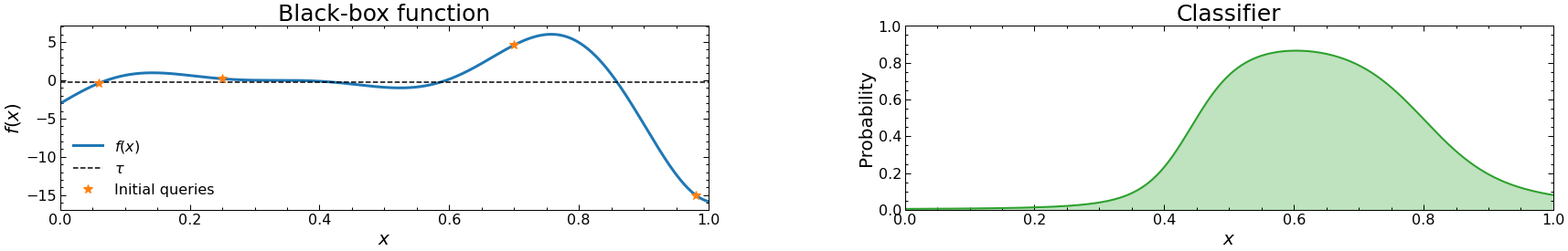
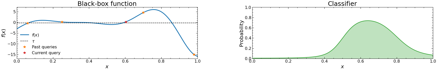
In Bayesian Optimization, one aims to maximize a black-box function $f$ from a series of queries. Denote the $n$ queries we get as $\mathcal{D}_n = \{(x_1, y_1), \ldots, (x_n, y_n)\}$. Often, a surrogate model $p(y | x, \mathcal{D}_n)$ is used to decide where we query next (i.e., $x_{n+1}$). This is done by finding the argmax of an acquisition function in the form of the expectation of some utility function: $$ \mathbb{E}_{y \sim p(y | x, \mathcal{D}_n)}[u(y; \tau)] = \int u(y; \tau) p(y | x, \mathcal{D}_n) \mathrm{d} y $$ where $\tau$ can be treated as a threshold. Common acquisition functions include:

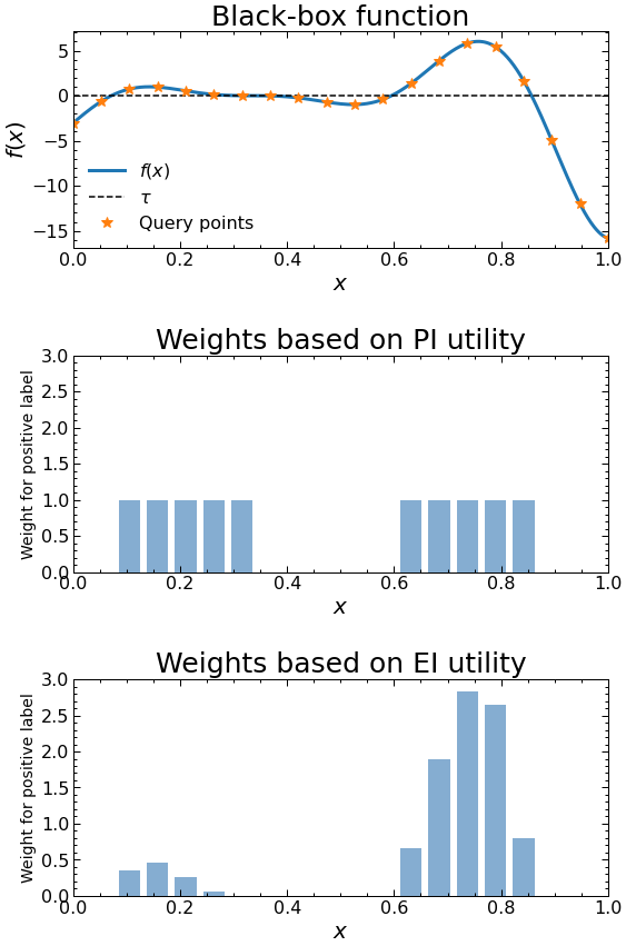
Probability of Improvement (PI): $u^{\mathrm{PI}}(y; \tau) := \mathbb{I}(y - \tau, 0)$, where $\mathbb{I}$ is the binary indicator function. This indicates whether $y$ is above or below the threshold $\tau$ or not.
Expected Improvement (EI): $u^{\mathrm{EI}}(y; \tau) := \max(y - \tau, 0)$. This indicates by how much $y$ is above the threshold $\tau$ (if it is below, then 0 is returned).

When the surrogate model is a GP, the expectations in PI and EI have analytical forms; however, this is not necessarily true for other utility functions.

Bayesian Optimization from Classification

While GPs are very flexible probabilistic models, they can be relatively slow when the number of queries is large, or lack representation capacity due to the underlying kernel function; these limitations could pose a problem when the search space is very high-dimenisonal. Instead, there can be relatively simple methods that can still produce good solutions, but without having to use probabilistic models.

For example, suppose that we have queried these initial points of the underlying function $f$ (see bottom left). Among the points, some have high $f(x)$ and others do not; we can draw a line here ($y = \tau$) as a decision boundary, where for every new point $x$ we want to predict the probability of $f(x)$ being over the line. We can then train a classifier over the observations to perform this task (see bottom right).

We can see that this classifier predicts high values closer to the point where the observed $f(x)$ is high. In fact, we can use the classifier as the acquisition function to guide us where to query the next point; it turns out to be quite reasonable, as it is close to where we have observed a high $f(x)$.

We can further repeat this process and observe that we have managed to find a pretty reasonable $f(x)$ in a couple of iterations.

Loading...

If we define any distribution over $x$, then this approach can be treated as trying to estimate the density ratio between $p(x | y > \tau)$ and $p(x | y < \tau)$; if this ratio for a particular $x$ is high, then we believe that it would have a high $f(x)$. This approach is therefore called "Bayesian Optimization with Ratio Estimation" (BORE), which uses a likelihood-free inference method to obtain the density ratio.

General acquisition functions from likelihood-free inference

The problem with the above approach is that it only considers whether $y$ is over the threshold $\tau$, but not by how much it is over $\tau$. Therefore, a query that is over the threshold by a massive amount is treated equally as one that is barely over it.

Can the classifier also take into account information that is beyond the binary indicator (over the threshold or not)?

In this paper, we propose a simple solution.

In the earlier case, the classifier is trained by treating every observation with equal weights.
We propose to instead reweight the "positive" queries (i.e., ones that are above the threshold) by its utility value $u(y, \tau)$. When we use the utility associated with the EI acquisition function, we will reweight the queries $(x_i, y_i)$ by $\max(y_i - \tau, 0)$.
Here, we place larger weights to queries with larger observation value, which is reasonable because the maxima is more likely to yield in their vincinity. If we have infinite data and modeling capacity, our learned classifier will converge to EI, unlike the one used in BORE (which will converge to PI).

The new weights are applied only to points that are over the threshold.

After we obtain the weights, the training loss is just standard weighted logistic regression. In PyTorch, this is simply written as:

loss = nn.BCEWithLogitsLoss(weight=weight)(target, label)

The reweighting can also be easily implemented in other standard machine learning frameworks like scikit-learn or XGBoost. Beyond the utility associated with the EI acquisition function, we can also use any non-negative utility function, which could be intractable with GPs.

As our method is able to learn an acquisition function for any non-negative utility via likelihood-free inference, we name our method Likelihood-Free Bayesian Optimization (LFBO). Like BORE, we use likelihood-free inference, but unlike it, we are able to learn a general expectation-based acquisition functions (instead of just density ratios).

Comparing different types of acquisition functions

Top: Closed-form acquisition functions in the form of expected utility often require certain utility functions (e.g., PI and EI) and certain surrogate models (e.g., GPs).
Middle: BORE uses simple, deterministic models (e.g., neural networks, decision trees) to model a density ratio with likelihood-free inference, but this limits its utility function to the one for PI.
Bottom: Our likelihood-free BO approach extends BORE to any non-negative utility function, including the one associated with EI and others whose expectations may not have a closed-form solution (e.g., EI with composite function).

Experimental results on real-world benchmarks

We compare our approach with a comprehensive set of state-of-the-art black-box optimization methods, including BORE, Tree-structured Parzen Estimator (TPE), Sequential Model-based Algorithm Configuration (SMAC), GP-based Expected Improvement and Random Search. Here, we use the utility function for EI in LFBO. We also conisder three types of models for BORE and LFBO: Multi-Layer Perceptrons (MLP), Gradient-boosted Trees (XGB), and Random Forests (RF). We report the immediate regret (i.e., the absolute error between the global minimum of each benchmark and the lowest function value observed so far) following previous work¹We note that in this work and BORE, the actual output from the black-box function is a random value from several possible ones (simulating noise in the optimization process), whereas the global minimum considers the expectation over the values. Therefore, a negative immediate regret is possible (and we would use the corresponding neural network for deployment). The flat vertical lines in our plots mean that the average immediate regret (across all the seeds) has become negative..

Neural network tuning

In HPOBench, we aim to find the optimal hyperparameter configurations for training a two-layer feed-forward neural networks on four popular UCI datasets. The configuration space includes batch size, initial learning rate, learning rate schedule, as well as layer-specific dropout rates, number of units and activation functions. For each dataset, HPOBench tabulates the mean squared errors of all 62,208 configurations.

Neural architecture search

In NAS-Bench-201, the network architecture is constructed as a stack of neural cells, each represented as a directed acyclic graph (DAG), and we focus on the design of the neural cell, \textit{i.e.}, assigning an operation to 6 edges of the DAG from a set of 5 operations. Similar to HPOBench, this dataset also provides a lookup table that tabulates the training results of all 15,625 possible configurations for three datasets.

We can see that our LFBO approach consistently achieves the best result across all the datasets, except on NAS-Bench-201-CIFAR-10 where the SMAC method is slightly better. Notably, with all three classifier implementations (MLP, RF and XGBoost), LFBO (EI) consistently outperforms its BORE counterparts except for Naval with MLP, which demonstrates the effectiveness of choosing EI as the acquisition function and the value of enabling EI in the likelihood-free scenario.

Experimental results on composite objective functions

Here, we consider the case of composite objective functions, where $f(x) = -\Vert h(x) - z_\star \Vert_2^2$ is based on a vector-valued black-box function $h(x)$ and $z_\star \in \mathbb{R}^d$$ is a vector observed from the real world. Compared to standard BO approaches that do not exploit this information, a grey-box BO method that explicitly models $h$ can make a much better sampling decision. In LFBO, we can easily take into account the structure of the problem in the classifier model (which we call "Composite LFBO"). Composite LFBO approach performs significantly better than regular GP and LFBO, while being on par with a composite GP approach.

BibTeX

@inproceedings{song2022a,
  title={A General Recipe for Likelihood-free Bayesian Optimization},
  author={Song*, Jiaming and Yu*, Lantao and Neiswanger, Willie and Ermon, Stefano},
  booktitle={International Conference on Machine Learning},
  year={2022}
}